Mathematica
1.安装
在网站Free Wolfram Engine for Developers找到对应自己电脑系统的安装包
我选择的是linux版本,这个是免费的开发者版本
然后会跳到一个注册界面,注册完成后记住账号密码,后续有用
下载完WolframEngine_12.2.0_LIN_CN.sh文件后,再命令行bash进行安装,注意需要sudo获得权限
sudo bash WolframEngine_12.2.0_LIN_CN.sh
接下来会提示安装的路径:
Enter the installation directory, or press ENTER to select
/usr/local/Wolfram/WolframEngine/12.2:
安装成功后,cd到这个安装路径
按照How do I specify which kernel WolframScript should use?操作进行配置
wolframscript -config WOLFRAMSCRIPT_KERNELPATH="/usr/local/Wolfram/WolframEngine/12.2/Executables/WolframKernel"
然后输入
wolframscript
此时需要输入Wolfram ID和Password,这就是之前注册的信息
完成后就来到Wolfram的计算环境,现在可以尽情探索了
输入Quit[]可退出
安装jupyterlab
sudo pip3 install jupyterlab
运行jupyter-lab
这时终端会弹出网址
http://localhost:8888/lab?token=9b7513e72a26836335c16e5f3d1ae1323117e5516ffeb2e0
http://127.0.0.1:8888/lab?token=9b7513e72a26836335c16e5f3d1ae1323117e5516ffeb2e0
在浏览器上登陆网址,就可以访问到jupyterlab
在WolframLanguageForJupyter中下载WolframLanguageForJupyter-0.9.2.paclet
在WolframEngine中输入wolframscript后
In[7]:= PacletInstall["./Downloads/WolframLanguageForJupyter-0.9.2.p
aclet"]

Out[7]= PacletObject[WolframLanguageForJupyter, 0.9.2, <>]

In[8]:= Needs["WolframLanguageForJupyter`"]

In[9]:= ConfigureJupyter["Add"]
这时再刷新http://127.0.0.1:8888/lab
就可以看到wolfram入口了
2.雕虫小技
出现报错
No valid password found.
Connection closed by WolframKernel.
The Wolfram Engine exited because of a license error: single machine process limit reached.
说明已经有引擎在运行了,需要先退出来原来的引擎,只允许单个的进程运行
可在命令行直接运行,如
wolframscript -code 2+2
也可通过Wolfram Cloud来计算
wolframscript -cloud -code 2+2
Mathematica 比起 Python 如今还有什么优势?
This open source project is for Mathematica (Wolfram Language) implementations of statistical and Machine Learning algorithms that can be used for data analysis, forecast, prediction, and recommendation systems.
如果输出表达式,可以在后面加上//TeXForm, 生成比较美观的输出,tex格式
In[15]:= x+1/y//TeXForm

Out[15]//TeXForm= x+\frac{1}{y}
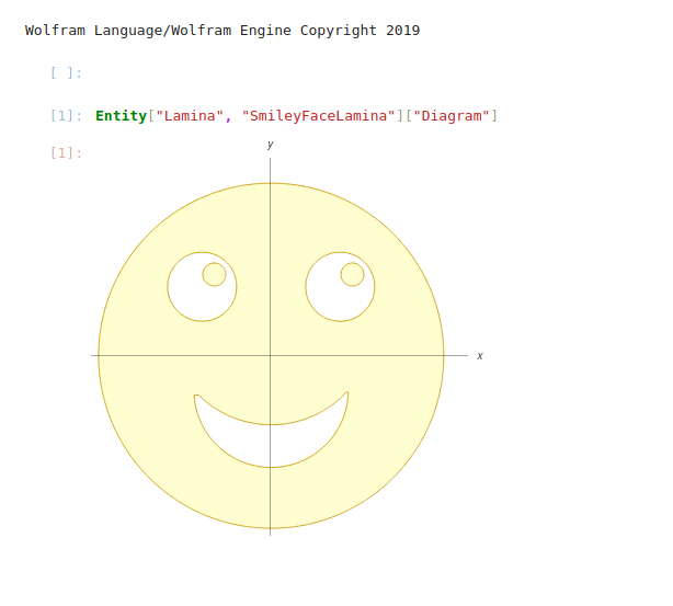
输入
Entity["Lamina", "SmileyFaceLamina"]["Diagram"]
可以看到输出有表情的图片了
检测一段文本的情感
wolframscript -code 'Classify[ "Sentiment", "That is too bad" ]'
用 Python 运行Wolfram 语言代码
安装 sudo pip3 install wolframclient
from wolframclient.evaluation import WolframLanguageSession
from wolframclient.language import wl, wlexpr
session = WolframLanguageSession()
计算列表的最小最大值
session.evaluate(wl.MinMax([1, -3, 0, 9, 5]))
运行脚本文件
mimmax.wls
l = {1, -3, 0, 9, 5};
y = MinMax[l];
Print[y];
运行wls文件
$ wolframscript -file mimmax.wls
output:
{-3, 9}
Cartoonise people in videos with neural networks, image/video processing
进行List的排序:
In[9]:= {4, 14, 5, 11, 12, 0, 6, 5, 1,  14, 29} //. {x1___, x2_, x3_, x4___} /;
x2 > x3 :> {x1, x3, x2, x4}

Out[9]= {0, 1, 4, 5, 5, 6, 11, 12, 14, 14, 29}
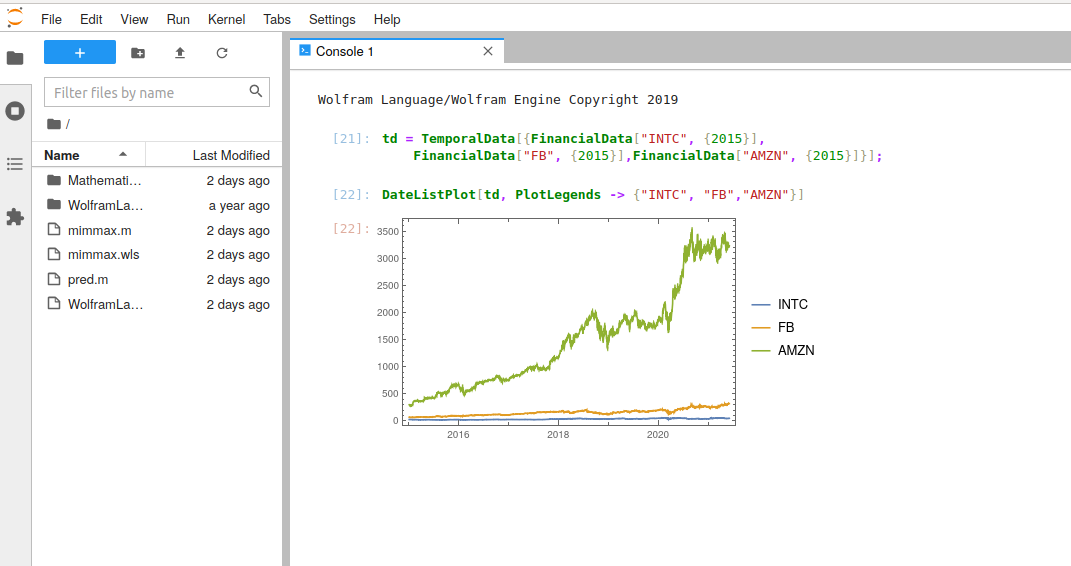
获取INTC,FB,AMZN 2015年以来的财务时序数据并画图
td = TemporalData[{FinancialData["INTC", {2015}],
    FinancialData["FB", {2015}],FinancialData["AMZN", {2015}]}];
DateListPlot[td, PlotLegends -> {"INTC", "FB","AMZN"}]
获取一个可用属性列表:
td["Properties"]
SparseArray在特定位置指定值
In[22]:= Normal[SparseArray[{3->x,4->y},5]]

Out[22]= {0, 0, x, y, 0}
f@x 方式:与 f[x] 方式等价,好处是避免使用方括号,提高代码的可读性。例如,f@g@h@x 的可读性要高于 f[g[h[x]]]。
音视频:
VideoGenerator — 根据图像、音频和任意函数生成视频
VideoIntervals — 找到视频中的兴趣区间
AnimatedImage — 根据文件或图像列表创建和表示动画图像
Wolfram Certified Level II Multiparadigm Data Science
Recommended Level II Certification Process:
Begin by studying the materials available in the Multiparadigm Data Science interactive course. Watch all 21 videos and pass the 4 quizzes in order to earn your certificate of course completion. Track your certification progress within the course by selecting Certification Overview at the bottom of the table of contents. Complete required exercises for Level I certification. Prepare for Level II certification by selecting a dataset from the list of Multiparadigm Data Science projects. Create your independent project notebook. Consult the grading rubric to ensure your project meets certification standards.
Pay the $395 certification fee and submit your project notebook. (Education customers pay $195; students pay $95.)
Wolfram Certified Level II Grading Rubric
1000以内能被3整除的数
In[4]:= Range[3,999,3]

Out[4]= {3, 6, 9, 12, 15, 18, 21, 24, 27, 30, 33, 36, 39, 42, 45, 48, 51, 54,

>    57, 60, 63, 66, 69, 72, 75, 78, 81, 84, 87, 90, 93, 96, 99, 102, 105,

>    108, 111, 114, 117, 120, 123, 126, 129, 132, 135, 138, 141, 144, 147,

>    150, 153, 156, 159, 162, 165, 168, 171, 174, 177, 180, 183, 186, 189,

>    192, 195, 198, 201, 204, 207, 210, 213, 216, 219, 222, 225, 228, 231,

>    234, 237, 240, 243, 246, 249, 252, 255, 258, 261, 264, 267, 270, 273,

>    276, 279, 282, 285, 288, 291, 294, 297, 300, 303, 306, 309, 312, 315,

>    318, 321, 324, 327, 330, 333, 336, 339, 342, 345, 348, 351, 354, 357,

>    360, 363, 366, 369, 372, 375, 378, 381, 384, 387, 390, 393, 396, 399,

>    402, 405, 408, 411, 414, 417, 420, 423, 426, 429, 432, 435, 438, 441,

>    444, 447, 450, 453, 456, 459, 462, 465, 468, 471, 474, 477, 480, 483,

>    486, 489, 492, 495, 498, 501, 504, 507, 510, 513, 516, 519, 522, 525,

>    528, 531, 534, 537, 540, 543, 546, 549, 552, 555, 558, 561, 564, 567,

>    570, 573, 576, 579, 582, 585, 588, 591, 594, 597, 600, 603, 606, 609,

>    612, 615, 618, 621, 624, 627, 630, 633, 636, 639, 642, 645, 648, 651,

>    654, 657, 660, 663, 666, 669, 672, 675, 678, 681, 684, 687, 690, 693,

>    696, 699, 702, 705, 708, 711, 714, 717, 720, 723, 726, 729, 732, 735,

>    738, 741, 744, 747, 750, 753, 756, 759, 762, 765, 768, 771, 774, 777,

>    780, 783, 786, 789, 792, 795, 798, 801, 804, 807, 810, 813, 816, 819,

>    822, 825, 828, 831, 834, 837, 840, 843, 846, 849, 852, 855, 858, 861,

>    864, 867, 870, 873, 876, 879, 882, 885, 888, 891, 894, 897, 900, 903,

>    906, 909, 912, 915, 918, 921, 924, 927, 930, 933, 936, 939, 942, 945,

>    948, 951, 954, 957, 960, 963, 966, 969, 972, 975, 978, 981, 984, 987,

>    990, 993, 996, 999}
清除在当前Mathematica进程中的所有定义:
Clear["Global`*"]
在v的各项之间交错插入x:
In[1]:= v = Range[5]

Out[1]= {1, 2, 3, 4, 5}

In[2]:= Riffle[v,x]

Out[2]= {1, x, 2, x, 3, x, 4, x, 5}
Table的用法
In[5]:= data = Table[i,{i,1,5},{j,1,4}]

Out[5]= {{1, 1, 1, 1}, {2, 2, 2, 2}, {3, 3, 3, 3}, {4, 4, 4, 4}, {5, 5, 5, 5}}

In[6]:= data = Table[j,{i,1,5},{j,1,4}]

Out[6]= {{1, 2, 3, 4}, {1, 2, 3, 4}, {1, 2, 3, 4}, {1, 2, 3, 4}, {1, 2, 3, 4}}

In[7]:= data = Table[i+j,{i,1,5},{j,1,4}]

Out[7]= {{2, 3, 4, 5}, {3, 4, 5, 6}, {4, 5, 6, 7}, {5, 6, 7, 8}, {6, 7, 8, 9}}
选出第二个列表中1所对应的元素
In[37]:= Pick[{a,b,c,d},{1,0,1,1},1]

Out[37]= {a, c, d}
求f[x]=x^2,x初值为2,重复迭代f[x]3次
In[42]:= Nest[#^2&,2,3]

Out[42]= 256
对上面进行同样的计算,但把大于10的中间结果作为后面列表展示出来
In[43]:= Reap[Nest[(If[#>10,Sow[#]];#^2)&,2,3]]

Out[43]= {256, 16}
从索引位置2开始每隔(3-1)=2个位置取值
In[51]:= Take[{a,b,c,d,e,f,g},{2,-1,3}]

Out[51]= {b, e}
里面参数添加外面层输入作为参数
In[53]:= Outer[f,{a,b},{c,d},{e,f}]

Out[53]= {{{f[a, c, e], f[a, c, f]}, {f[a, d, e], f[a, d, f]}},

>    {{f[b, c, e], f[b, c, f]}, {f[b, d, e], f[b, d, f]}}}
将第3列与第2列互换
In[56]:= x = Array[a,{2,2,2}]

Out[56]= {{{a[1, 1, 1], a[1, 1, 2]}, {a[1, 2, 1], a[1, 2, 2]}},

>    {{a[2, 1, 1], a[2, 1, 2]}, {a[2, 2, 1], a[2, 2, 2]}}}

In[57]:= Transpose[x,{1,3,2}]

Out[57]= {{{a[1, 1, 1], a[1, 2, 1]}, {a[1, 1, 2], a[1, 2, 2]}},

>    {{a[2, 1, 1], a[2, 2, 1]}, {a[2, 1, 2], a[2, 2, 2]}}}
创建一个带状矩阵
In[70]:= SparseArray[{Band[{1,1}]-> x,Band[{2,1}]->y},{5,5}]

Out[70]= SparseArray[<9>, {5, 5}]

In[71]:= % //MatrixForm

Out[71]//MatrixForm= x   0   0   0   0

                     y   x   0   0   0

                     0   y   x   0   0

                     0   0   y   x   0

                     0   0   0   y   x
生成带状对角矩阵
In[11]:= Normal[SparseArray[{i_,j_} /;Abs[i-j]<2->3,{5,5}]]

Out[11]= {{3, 3, 0, 0, 0}, {3, 3, 3, 0, 0}, {0, 3, 3, 3, 0}, {0, 0, 3, 3, 3},

>    {0, 0, 0, 3, 3}}

In[12]:= % //MatrixForm

Out[12]//MatrixForm= 3   3   0   0   0

                     3   3   3   0   0

                     0   3   3   3   0

                     0   0   3   3   3

                     0   0   0   3   3
定义一个函数,提取常数因子:
In[20]:= f[c_ x_, x_] := c f[x, x] /; FreeQ[c, x]

In[21]:= {f[3 x, x], f[a x, x], f[(1 + x) x, x]}

Out[21]= {3 f[x, x], a f[x, x], f[x (1 + x), x]}
保留已有值的函数
In[1]:= f[x_]:=f[x] = f[x-1]+f[x-2]

In[2]:= f[0]=f[1]=1

Out[2]= 1

In[3]:= ?f

Out[3]= Global`f
        f[1] = 1

        f[0] = 1

        f[x_] := f[x] = f[x - 1] + f[x - 2]


In[4]:= f[5]

Out[4]= 8

In[5]:= ?f

Out[5]= Global`f
        f[1] = 1

        f[0] = 1

        f[2] = 2

        f[3] = 3

        f[4] = 5

        f[5] = 8

        f[x_] := f[x] = f[x - 1] + f[x - 2]


In[6]:= f[5]

Out[6]= 8
求n项连乘多项式的i次项系数
In[7]:= exprod[n_]:=Expand[Product[x+i,{i,1,n}]]

In[8]:= exprod[5]

                           2       3       4    5
Out[8]= 120 + 274 x + 225 x  + 85 x  + 15 x  + x

In[9]:= cex[n_,i_]:=(t=exprod[n];Coefficient[t,x^i])

In[10]:= cex[5,3]

Out[10]= 85
产生新符号时显示一个信息
In[9]:= On[General::newsym]

In[10]:= sin[k]
               General::newsym: Symbol sin is new.

                                                  General::newsym: Symbol k is new.


Out[10]= sin[k]
给出字符串中所有相同字符组成的对
In[1]:= StringCases["abbcbccaabbabccaa",x_~~x_]

Out[1]= {bb, cc, aa, bb, cc, aa}
绘制网格圆
Graphics3D[{PointSize@Medium,
  Map[{Blend[{Green, Red}, (Mean@*Flatten @@ # + 1)/2], #} &,
   MeshPrimitives[DiscretizeRegion@Sphere[], #] & /@ {0, 1}, {2}]},
 Boxed -> False]
找出2^500中数字0的所有位置
In[15]:= Flatten[Position[IntegerDigits[2^500], 0]]

Out[15]= {7, 9, 19, 20, 44, 47, 50, 65, 75, 88, 89, 96, 103, 115, 116, 119, 120, 137}
应用于单个点的置换:
In[1]:= PermutationReplace[3, Cycles[{{1, 3, 2}}]]

Out[1]= 2
表示计算3映射到后面的元素
双点”x..” 或 Repeated[x]函数表示一个或多个表达式的序列,每个表达式匹配模式 x。例如,
{{}, {a, a}, {a, b}, {a, a, a}, {a}} /. {a ..} -> x
结果为
{{}, x, {a, b}, x, x}。
注意:当x..中的x元素为数字时,要加入空格避免与小数点混淆。例如 0 ..
自动构建列表
Table函数:按照指定次数和指定值,生成某个函数的列表。例如,Table[x,5],生成{x,x,x,x,x};Table[a[n],{n,5}],生成{a[1], a[2], a[3], a[4], a[5]}。这个函数的用途很广泛,使用频率很高。
对列表元素排序
In[12]:= FixedPointList[(# /. {x___, b_, a_, y___} /; b > a -> {x, a, b, y}) &,
{4, 5, 1, 3, 2}]

Out[12]= {{4, 5, 1, 3, 2}, {4, 1, 5, 3, 2}, {1, 4, 5, 3, 2}, {1, 4, 3, 5, 2},

>    {1, 3, 4, 5, 2}, {1, 3, 4, 2, 5}, {1, 3, 2, 4, 5}, {1, 2, 3, 4, 5},

>    {1, 2, 3, 4, 5}}
利用ListLinePlot可视化上述结果。代码:ListLinePlot[%]
以数学符号形式查看矩阵
In[1]:= matrices =  RandomInteger[2,{5,2,2}]

Out[1]= {{{1, 0}, {2, 0}}, {{1, 1}, {2, 0}}, {{1, 0}, {2, 2}},

>    {{1, 1}, {1, 2}}, {{2, 2}, {1, 0}}}

In[2]:= MatrixForm /@matrices

Out[2]= {1   0, 1   1, 1   0, 1   1, 2   2}

         2   0  2   0  2   2  1   2  1   0
属于符号怎么打
q=e Exp[I t];
cq=ComplexExpand[1/(1-q)];
Simplify[Re[cq],Assumptions->{e,t} \[Element] Reals] (*Imag part = 0*)Simplify[Im[cq],Assumptions->{e,t} \[Element] Reals] (*Imag part = 0*)
绘制三维心形图并导出为图片
Export["heart.jpg",
 ContourPlot3D[(x^2 + (9 y^2)/4 + z^2 - 1)^3 -
    x^2 z^3 - (9 y^2 z^3)/80 == 0, {x, -1.5, 1.5}, {y, -1.5,
   1.5}, {z, -1.5, 1.5}, Boxed -> False, Axes -> False, Mesh -> None,
  ContourStyle -> Red, PlotPoints -> 90]]

3.数学领域
组合
Mathematica的Combinatorica程序包来研究分拆
Sort orders symbols by their names, and in the event of a tie, by their contexts.
in the event of a tie 如遇平局
Sort by comparing the second part of each element:
In[2]:= Sort[{{a, 2}, {c, 1}, {d, 3}}, #1[[2]] < #2[[2]] &]

Out[2]= {{c, 1}, {a, 2}, {d, 3}}
Use NumericalOrder to allow complex numbers and number-like expressions:
In[4]:= Sort[{Yesterday, Tomorrow, Today}, NumericalOrder]

Out[4]= {DateObject[{2021, 5, 18}, Day, Gregorian, 8.],

>    DateObject[{2021, 5, 19}, Day, Gregorian, 8.],

>    DateObject[{2021, 5, 20}, Day, Gregorian, 8.]}
代数
x = {1,2}^T,A = {{2,a},{3,4}},B={{6,4},{7,5}},x^T.A.x = det B,求a值
In[4]:= Solve[{1,2}.{{2,a},{3,4}}.{{1},{2}}==Det[{{6,4},{7,5}}],a]

Out[4]= {{a -> -11}}
对矩阵特征值进行化简
In[5]:= Simplify[Det[{{x1^2,x1,1},{x2^2,x2,1},{x3^2,x3,1}}]]

Out[5]= (x1 - x2) (x1 - x3) (x2 - x3)
复数转指数函数表示
In[139]:= y[r_] =TrigToExp[Abs[r] (Cos[x]+I Sin[x])] /. (x->Arg[r])

           I Arg[r]
Out[139]= E         Abs[r]

In[140]:= y[1+I]

                   I/4 Pi
Out[140]= Sqrt[2] E

In[141]:= y[2+I]

                   I ArcTan[1/2]
Out[141]= Sqrt[5] E
An expression that reduces to 0 under the action of the infinitesimal generator is called an invariant of the group.
如何验证invariant
In[11]:= m=x*Cos[t]+y*Sin[t];

In[12]:= n=y*Cos[t]-x*Sin[t];

In[13]:= Series[m ,{t, 0, 1}] // Normal

Out[13]= x + t y

In[14]:= Series[n ,{t, 0, 1}] // Normal

Out[14]= -(t x) + y

In[15]:= v=(y*D[#,x]-x*D[#,y])&;

In[19]:= invariant=x^2+y^2;

In[20]:= v[invariant]

Out[20]= 0

In[21]:= invariant2=x^2+y^3;

In[22]:= v[invariant2]

                      2
Out[22]= 2 x y - 3 x y
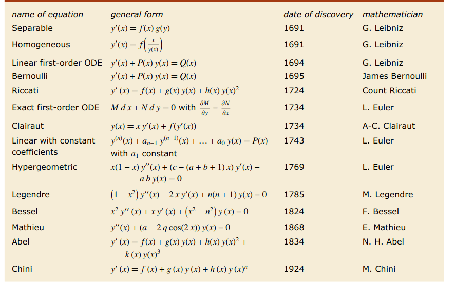
微分方程
解微分方程时得到解中含有形如K[1]的未知变量时可用换元法替代为自然记号
In[1]:= sol = DSolve[y'[x]+y[x]==Q[x],y[x],x]

                                              K[1]
                  C[1]   Inactive[Integrate][E     Q[K[1]], {K[1], 1, x}]
Out[1]= {{y[x] -> ---- + ------------------------------------------------}}
                    x                            x
                   E                            E

In[2]:= sol /. {K[1] -> t}

                                              t
                  C[1]   Inactive[Integrate][E  Q[t], {t, 1, x}]
Out[2]= {{y[x] -> ---- + ---------------------------------------}}
                    x                       x
                   E                       E
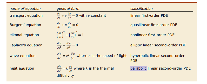
At this stage of development, DSolve typically only works with PDEs having two independent variables
将初值条件和微分方程分开来写然后联合求解并画出3D图
In[25]:= Clear[x, y, z, t ]

In[26]:= linearsystem={x'[t] == x[t]-4*y[t]+1,y'[t] == 4*x[t]+y[t],z'[t] == z[t]
};

In[27]:= initialvalues={x[0]==2,y[0]==-1,z[0]==1};

In[28]:= sol=DSolve[Join[linearsystem, initialvalues],{x, y, z},t]

Out[28]= {{x ->

                         t                    2       t                    2
                     35 E  Cos[4 t] - Cos[4 t]  + 21 E  Sin[4 t] - Sin[4 t]
>      Function[{t}, -------------------------------------------------------],
                                               17

>     y -> Function[{t},

              t                      2       t                      2
         -21 E  Cos[4 t] + 4 Cos[4 t]  + 35 E  Sin[4 t] + 4 Sin[4 t]
>        ------------------------------------------------------------],
                                      17

                          t
>     z -> Function[{t}, E ]}}

In[29]:= ParametricPlot3D[Evaluate[{x[t], y[t], z[t]} /. sol], {t,-7,-3},PlotRan
ge -> All]
遇到微分方程的隐式解时可做转换
In[44]:= sol = DSolve[Derivative[2][y][x]+y[x]*Derivative[1][y][x]^4 == 0,y,x]

Out[44]= {{y ->

                                                                    2
>      Function[{x}, InverseFunction[C[1] Log[#1 + Sqrt[-2 C[1] + #1 ]] -

                                2
            #1 Sqrt[-2 C[1] + #1 ]
>           ---------------------- & ][x + C[2]]]},
                      2

>    {y -> Function[{x}, InverseFunction[-(C[1]

                                                                    2
                                         2      #1 Sqrt[-2 C[1] + #1 ]
>              Log[#1 + Sqrt[-2 C[1] + #1 ]]) + ---------------------- & ][
                                                          2

>        x + C[2]]]}}

In[45]:= soly = y[x] /. sol[[1]]

                                                        2
Out[45]= InverseFunction[C[1] Log[#1 + Sqrt[-2 C[1] + #1 ]] -

                            2
        #1 Sqrt[-2 C[1] + #1 ]
>       ---------------------- & ][x + C[2]]
                  2

In[47]:= implicitequation = (Head[soly][[1]][y[x]] == soly[[1]])

                                            2
Out[47]= C[1] Log[y[x] + Sqrt[-2 C[1] + y[x] ]] -

                              2
      y[x] Sqrt[-2 C[1] + y[x] ]
>     -------------------------- == x + C[2]
                  2
用GeneratedParameters改变微分方程解中未定义的参数
In[53]:= DSolve[y'[x]+y[x] ==1,y[x],x,GeneratedParameters ->P]

                       P[1]
Out[53]= {{y[x] -> 1 + ----}}
                         x
                        E


In[56]:= DSolve[y''[x]+y[x] ==1,y[x],x,GeneratedParameters -> (const[#] &)]

Out[56]= {{y[x] -> 1 + const[1] Cos[x] + const[2] Sin[x]}}
如果得不到方程的解,可以尝试互换自变量和因变量
In[58]:= Clear["Global`*"]

In[59]:= DSolve[y'[x] ==1 / (x-y[x]) && y[0] ==1,y,x]

Solve::ifun: Inverse functions are being used by Solve, so some solutions may not be
     found; use Reduce for complete solution information.

DSolve::bvnul: For some branches of the general solution, the given boundary
    conditions lead to an empty solution.

Out[59]= {}

In[60]:= DSolve[x'[y] ==(x[y]-y) && x[1] ==0,x,y]

                                     y
                              E - 2 E  + E y
Out[60]= {{x -> Function[{y}, --------------]}}
                                    E
画图给坐标轴打标题
In[1]:= exactsolution=DSolve [{D[D[xe[t],t],t]+w0^2 xe[t]==0,xe[0]==0,xe'[0]==1}
,xe[t],t]

                   Sin[t w0]
Out[1]= {{xe[t] -> ---------}}
                      w0

In[3]:= Plot[{xe[t]/.exactsolution /. w0 ->1},{t,0,10},PlotStyle -> Blue, AxesLa
bel -> {"t","x(t)"}]

Out[3]= -Graphics-
Finally, we will create a movie with the trajectory graphs of a particle. We will take uniform circular motion, so x(t) =Acos(ωt) and y(t) =Asin(ωt). Choosing A=ω= 1, we can create a movie with the following commands
x[t_] := A*Cos[w*t]; y[t_] := A*Sin[w*t]; A = 1;w= 1;  tRange = Range [0.001 ,  20*Pi, 20*Pi/500];
For[k = 1, k  <= Length[tRange], k++, tk = tRange[[k]]; xk = x[tk]; yk = y[tk];movieVector[k] =Show[Graphics[{AbsolutePointSize[15], Green ,Point[{xk, yk}]},PlotRange  -> {{-1.1, 1.1}, {-1.1, 1.1}}] ,ParametricPlot [{x[t], y[t]}, {t, 0, tk},PlotStyle  -> Red ,PlotRange  -> {{-1.1, 1.1}, {-1.1, 1.1}}] ,AxesLabel  -> {"x","y"},PlotLabel  -> StringJoin["t=", ToString[N[tk]]]]]
M = Table[movieVector[k], {k, 1, 500}];
fileName ="FilmeMathematica.avi";
Export[fileName , M]
Directory []
随机过程
泊松过程比较参数不同的路径(学习其中图标的用法):
In[1]:= sample[\[Mu]_] := (SeedRandom[3];
  RandomFunction[PoissonProcess[\[Mu]], {0, 20}])

In[2]:= pars = {.6, 1, 3.5};

In[3]:= ListStepPlot[sample[#], Filling -> Axis,
   PlotLabel -> StringJoin["\[Lambda] = ", ToString[#]]] & /@ pars
顾客按照每小时 4 个的泊松抵达率到达一个商店. 假定商店早上 9 点开门,求到早上 9 点半恰好已有一个顾客到达的概率:
In[6]:= arrivalProcess = PoissonProcess[4];
In[7]:= Probability[x[1/2] == 1, x \[Distributed] arrivalProcess]

        2
Out[7]= --
         2
        E

In[8]:= Probability[x[1/2] == 1, x \[Distributed] arrivalProcess];

In[9]:= N[%]

Out[9]= 0.270671
消息记录设备收到查询的过程服从抵达率为每分钟 15 条的泊松过程. 求在 1 分钟时间段内,前 10 秒钟有 3 条查询,最后 15 秒有 2 条查询的概率:
In[11]:= \[Lambda] = 15/60;
In[12]:= arrivalProcess = PoissonProcess[\[Lambda]];
在前 10 秒钟内有 3 条查询到达的概率:
In[13]:= p1 = NProbability[x[10] == 3, x \[Distributed] arrivalProcess]

Out[13]= 0.213763
由于事件是独立的,最后 15 秒与前 15 秒是一样的:
In[14]:= p2 = NProbability[x[15] == 2, x \[Distributed] arrivalProcess]
Out[14]= 0.165359
由于事件的独立性,两个概率相乘可得所求概率:
In[15]:= p1 p2

Out[15]= 0.0353477
你正在拨打热线电话,被告知去掉正在通话的人,你排在第 56 位,打电话的人按速率每小时 2 个的泊松过程离开,求你需要等候超过 30 分钟的概率:
In[16]:= callServiceProcess = PoissonProcess[2];

In[17]:= NProbability[x[30] < 56, x \[Distributed] PoissonProcess[2]]

Out[17]= 0.285491
旅客从早上 6 点开始,陆续到达一个公交车站,服从抵达率为每二分钟一个的泊松过程. 如果公交车的发车服从均值为 15 分钟的指数分布,求早上 6 点后从车站驶离的第一辆公交车上乘客数目的均值和方差:
In[19]:= \[Mu] = 1/2;

In[20]:= arrivalProcess = PoissonProcess[\[Mu]];

In[21]:= traveler\[ScriptCapitalD] =
 ParameterMixtureDistribution[arrivalProcess[\[Mu] t],
  t \[Distributed] ExponentialDistribution[1/15]]

                               4
Out[21]= GeometricDistribution[--]
                               19

In[22]:= {Mean[traveler\[ScriptCapitalD]],
  Variance[traveler\[ScriptCapitalD]]} // N

Out[22]= {3.75, 17.8125}
早上 6 点 15 分驶离的一辆有 20 个座位的公交车上乘客数量的平均值:
In[23]:= NExpectation[Min[x[15], 20], x \[Distributed] PoissonProcess[\[Mu]]]

Out[23]= 7.49994
出现在一个抛光镜面上的瑕疵的数目为泊松随机变量.一个镜子的表面积为 8.54 cm^2,无瑕疵的概率为 0.91. 使用同样的工艺制作另一面面积为 17.50 cm^2 的镜子. 求这个较大的镜子上不出现瑕疵的概率:
In[25]:= flawProcess = PoissonProcess[\[Lambda]];
根据较小镜子的信息求出泊松参数:
In[26]:= flawProcess = (flawProcess /.
    Solve[Probability[x[8.54] == 0, x \[Distributed] flawProcess] ==
       0.91, \[Lambda]][[1]]) // Quiet

Out[26]= PoissonProcess[0.0110434]
较大的镜子上不出现瑕疵的概率:
In[27]:= Probability[x[17.50] == 0, x \[Distributed] flawProcess]

Out[27]= 0.824268
灯泡的寿命是均值为 200 天的指数分布. 灯泡坏了之后,管理员会立即将它换掉. 此外,作为预防措施,还有一个修理工按泊松抵达率 0.01 时常过来检查并替换灯泡. 求灯泡被替换的平均天数:
In[29]:= \[Lambda] = 1/200 + 1/100;

In[30]:= bulbReplacementProcess = PoissonProcess[\[Lambda]];

In[31]:= 1/\[Lambda] // Round

Out[31]= 67
夜间,车辆在双向隔离的高速公路上行驶,该过程是一个速率为每个方向每分钟2辆车的泊松过程. 由于一次事故,某个方向的交通被暂时终止. 假定 60% 的车辆是小汽车,30% 是卡车,10% 是半拖车. 另外还假设小汽车的长度是 5 米,卡车的长度是 10 米,半拖车的长度是 20 米. 求事发后多久有 10% 的概率,累积车辆的长度超过 1 公里:
In[1]:= circulationProcess = PoissonProcess[2];

In[2]:= sampleQueue = RandomFunction[circulationProcess, {0, 40}]

Out[2]= TemporalData[<<1>>]

In[3]:= averageLength = (0.6*5 + 0.3*10 + 0.1*20);

In[4]:= sampleQueueLength = averageLength*sampleQueue

Out[4]= TemporalData[<<1>>]

In[5]:= queueLength = averageLength*x[t];

In[6]:= t /. FindRoot[
   Probability[queueLength > 1000,
     x \[Distributed] circulationProcess] == 1/10, {t, 40}][[1]]

Out[6]= 55.9228
优化
求解非线性规划问题
利用 Minimize,能够产生一个精确的解
In[1]:= Minimize[{x - y, -3 x^2 + 2 x y - y^2 >= -1}, {x, y}]

Out[1]= {-1, {x -> 0, y -> 1}}
数值化地解同样的问题
In[2]:= NMinimize[{x - y, -3 x^2 + 2 x y - y^2 >= -1}, {x, y}]

                               -10
Out[2]= {-1., {x -> -4.72886 10   , y -> 1.}}
FindMinimum 数值化地求一个局部最小值
In[3]:= FindMinimum[{x - y, -3 x^2 + 2 x y - y^2 >= -1}, {x, y}]

                               -10
Out[3]= {-1., {x -> -4.72886 10   , y -> 1.}}
NMinimize 和 NMaximize 执行好几种算法用以求约束全局最优解. 这些方法具有足够的灵活性,以处理不可微或连续,并且不容易被局部最优解捕捉的函数.
In[4]:= NMaximize[Sin[x + y] - x^2 - y^2, {x, y}]

Out[4]= {0.400489, {x -> 0.369543, y -> 0.369543}}
In[5]:= NMinimize[{x^2 + (y - .5)^2, y >= 0 && y >= x + 1}, {x, y}]

Out[5]= {0.125, {x -> -0.25, y -> 0.75}}
划定一个变量的定义域时用 Element ,例如,Element[x,Integers] 或者 x∈Integers
In[7]:= NMinimize[{(x - 1/3)^2 + (y - 1/3)^2, x \[Element] Integers}, {x, y}]

Out[7]= {0.111111, {x -> 0, y -> 0.333333}}
采用 RandomSearch 来寻找极小值:
In[17]:= f = E^Sin[50 x] + Sin[60 E^y] + Sin[70 Sin[x]] + Sin[Sin[80 y]] -
Sin[10 (x + y)] + 1/4 (x^2 + y^2)

                       2    2
          Sin[50 x]   x  + y            y
Out[17]= E          + ------- + Sin[60 E ] - Sin[10 (x + y)] +
                         4

>    Sin[70 Sin[x]] + Sin[Sin[80 y]]

In[19]:= NMinimize[f, {x, y}, Method -> "RandomSearch" ]

Out[19]= {-2.38708, {x -> -0.124868, y -> 0.290932}}

In[20]:= NMinimize[f, {x, y}, Method -> {"RandomSearch", "SearchPoints"->250} ]

Out[20]= {-3.14408, {x -> -0.0231678, y -> -0.494213}}
这里通过利用 DifferentialEvolution 将单位圆盘里的函数最小化:
In[22]:= NMinimize[{100 (y - x^2)*2 + (1 - x)^2, x^2 + y^2 <= 1}, {x, y}, Method
 -> "DifferentialEvolution"]

Out[22]= {-249.982, {x -> 0.866248, y -> -0.499614}}
模拟退火算法是一个简单的随机函数最小化算法. 这是从退火的物理过程得到启发的. 退火时,金属物体被加热到很高的温度并且慢慢冷却. 这个过程使金属的原子结构最终形成于一个较低的能量状态,从而成为更强硬的金属. 利用优化术语,退火使结构脱离局部最小值,探索并达到一个更好的,可望是全局的的最小值.
用 SimulatedAnnealing 对一个具有两个变量的函数最小化:
In[24]:= NMinimize[{100 (y - x^2)*2 + (1 - x)^2, -2.084 <= x <= 2.084 && -2.084
<= y <= 2.084}, {x, y}, Method -> "SimulatedAnnealing"]

Out[24]= {-1284.24, {x -> 2.084, y -> -2.084}}
这里利用 RandomSearch 将单位圆盘里的函数最小化:
In[26]:= NMinimize[{100 (y - x^2)*2 + (1 - x)^2, x^2 + y^2 <= 1}, {x, y}, Method
 -> "RandomSearch"]

Out[26]= {-249.982, {x -> 0.866248, y -> -0.499614}}
这里采用非线性内点法来寻找平方和的最小值:
In[28]:= n = 10;

In[29]:= f = Sum[(x[i] - Sin[i])^2, {i, 1, n}]

                         2                   2                   2
Out[29]= (-Sin[1] + x[1])  + (-Sin[2] + x[2])  + (-Sin[3] + x[3])  +

                     2                   2                   2
>    (-Sin[4] + x[4])  + (-Sin[5] + x[5])  + (-Sin[6] + x[6])  +

                     2                   2                   2
>    (-Sin[7] + x[7])  + (-Sin[8] + x[8])  + (-Sin[9] + x[9])  +

                       2
>    (-Sin[10] + x[10])

In[30]:= c = Table[-0.5 < x[i] < 0.5, {i, n}]

Out[30]= {-0.5 < x[1] < 0.5, -0.5 < x[2] < 0.5, -0.5 < x[3] < 0.5,

>    -0.5 < x[4] < 0.5, -0.5 < x[5] < 0.5, -0.5 < x[6] < 0.5,

>    -0.5 < x[7] < 0.5, -0.5 < x[8] < 0.5, -0.5 < x[9] < 0.5,

>    -0.5 < x[10] < 0.5}

In[31]:= v = Array[x, n]

Out[31]= {x[1], x[2], x[3], x[4], x[5], x[6], x[7], x[8], x[9], x[10]}

In[33]:= Timing[NMinimize[{f, c}, v, Method -> { "RandomSearch",Method -> "Inter
iorPoint"}]]

Out[33]= {10.892, {0.82674, {x[1] -> 0.5, x[2] -> 0.5, x[3] -> 0.14112,

>      x[4] -> -0.5, x[5] -> -0.5, x[6] -> -0.279416, x[7] -> 0.5,

>      x[8] -> 0.5, x[9] -> 0.412118, x[10] -> -0.5}}}
参考:
- TeXForm Output in JupyterLab
- 给Anaconda的Jupyter notebook笔记本安装Wolfram engine核心
- Smiley Face using parametric equations
- Ubuntu 18.04 服务器安装 JupyterLab
- Wolfram Engine使用+Jupyter协作
- 用于命令行的 WolframScript
- Wolfram Language (Mathematica) 学习笔记
- 如何学习mathematica
- Project Euler 1~50
- Mathematica中的约束最优化问题/遗传算法/退火算法
- 你的爱,用数学公式告诉她(他)